Author(s)
Tyler Sutterley, Hannah Besso, Scott Henderson, David Shean
Existing Notebooks
Learning Outcomes
Review fundamental concepts of geospatial coordinate reference systems (CRS)
Learn how to access CRS metadata
Learn basic coordinate transformations relevant to ICESat-2
import os
import pyproj
import warnings
import numpy as np
import rioxarray
import xarray as xr
import earthaccess
import geodatasets
import geopandas as gpd
import shapely.geometry
import matplotlib.pyplot as plt
import matplotlib.colors as mcolors
from mpl_toolkits import mplot3d
warnings.filterwarnings('ignore')
AWS_DEFAULT_REGION = os.environ.get('AWS_DEFAULT_REGION', '')

%matplotlib inline
In this notebook, we will explore coordinate systems, map projections, geophysical concepts and available geospatial software tools.
We’re going to use geopandas, xarray, and matplotlib for visualization.
geopandas is built on top of other great computing and geospatial tools, which will make our lives easier on this notebook.
- numpy: Scientific Computing Tools For Python
- pandas: Python Data Analysis Library
- shapely: PostGIS-ish operations outside a database context for Python
- GEOS: geometry, spatial operations
- GDAL/OGR: Pythonic interface to the Geospatial Data Abstraction Library (GDAL)
- fiona: Python wrapper for vector data access functions from the OGR library
- PROJ: cartographic projection and coordinate transformation library
- pyproj: Python interface to PROJ library
Let’s Start by Making a Map
### geopandas vector data from geodatasets
world = gpd.read_file(geodatasets.get_path('naturalearth.land'))
world.head()fig,ax1 = plt.subplots(num=1, figsize=(10,4.55))
minlon,maxlon,minlat,maxlat = (-180,180,-90,90)
world.plot(ax=ax1, color='0.8', edgecolor='none')
# set x and y limits
ax1.set_xlim(minlon,maxlon)
ax1.set_ylim(minlat,maxlat)
ax1.set_aspect('equal', adjustable='box')
# add x and y labels
ax1.set_xlabel('Longitude')
ax1.set_ylabel('Latitude')
# adjust subplot and show
fig.subplots_adjust(left=0.06,right=0.98,bottom=0.08,top=0.98)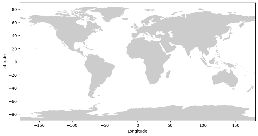
Geographic Coordinate Systems
Locations on Earth are usually specified in a geographic coordinate system consisting of
- Longitude specifies the angle east and west from the Prime Meridian (102 meters east of the Royal Observatory at Greenwich)
- Latitude specifies the angle north and south from the Equator
The map above projects geographic data from the Earth’s 3-dimensional geometry on to a flat surface. The three common types of projections are cylindric, conic and planar. Each type is a different way of flattening the Earth’s geometry into 2-dimensional space.
| Cylindric | Conic | Planar |
|---|---|---|
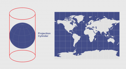 | 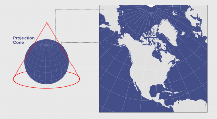 | 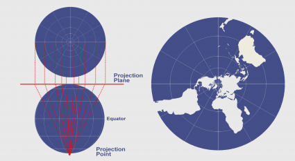 |
The above map is in an Equirectangular Projection (Plate Carrée), where latitude and longitude are equally spaced. Equirectangular is cylindrical projection, which has benefits as latitudes and longitudes form straight lines.
To illustrate distortion on this map below 👇, we’ve colored the normalized grid area at different latitudes below:
fig,ax1 = plt.subplots(num=1, figsize=(10.375,5.0))
minlon,maxlon,minlat,maxlat = (-180,180,-90,90)
dlon,dlat = (1.0,1.0)
longitude = np.arange(minlon,maxlon+dlon,dlon)
latitude = np.arange(minlat,maxlat+dlat,dlat)
# calculate and plot grid area
gridlon,gridlat = np.meshgrid(longitude, latitude)
im = ax1.imshow(np.cos(gridlat*np.pi/180.0),
    extent=(minlon,maxlon,minlat,maxlat),
    interpolation='nearest',
    cmap=plt.get_cmap('plasma'),
    origin='lower')
# add coastlines
world.plot(ax=ax1, color='none', edgecolor='black')
# set x and y limits
ax1.set_xlim(minlon,maxlon)
ax1.set_ylim(minlat,maxlat)
ax1.set_aspect('equal', adjustable='box')
# add x and y labels
ax1.set_xlabel('Longitude')
ax1.set_ylabel('Latitude')
# add colorbar
cbar = plt.colorbar(im, cax=fig.add_axes([0.92, 0.08, 0.025, 0.90]))
cbar.ax.set_ylabel('Normalized Grid Area')
cbar.solids.set_rasterized(True)
# adjust subplot and show
fig.subplots_adjust(left=0.06,right=0.9,bottom=0.08,top=0.98)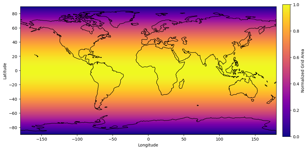
The Components of a Coordinate Reference System (CRS):
- Projection Information: the mathematical equation used to flatten objects that are on a round surface (e.g. the earth) so you can view them on a flat surface (e.g. your computer screens or a paper map).
- Coordinate System: the X, Y, and Z grid upon which your data is overlaid and how you define where a point is located in space.
- Horizontal and vertical units: The units used to define the grid along the x, y (and z) axis.
- Datum: A modeled version of the shape of the earth which defines the origin used to place the coordinate system in space.
👆 Borrowed from Earth Data Science Coursework
Map Projections
There is no perfect projection for all purposes
Not all maps are good for ocean or land navigation
Not all projections are good for polar mapping
Every projection will distort either shape, area, distance or direction:
- conformal projections minimize distortion in shape
- equal-area projections minimize distortion in area
- equidistant projections minimize distortion in distance
- true-direction projections minimize distortion in direction
While there are projections that are better suited for specific purposes, choosing a map projection is a bit of an art 🦋
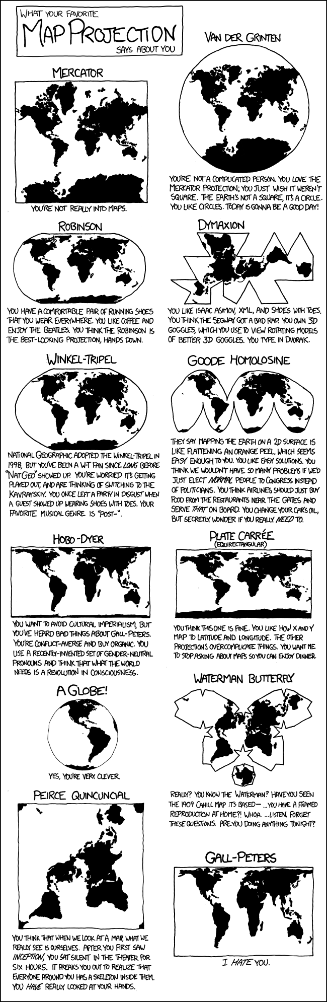
👆 Obligatory xkcd
world.crs<Geographic 2D CRS: EPSG:4326>
Name: WGS 84
Axis Info [ellipsoidal]:
- Lat[north]: Geodetic latitude (degree)
- Lon[east]: Geodetic longitude (degree)
Area of Use:
- name: World.
- bounds: (-180.0, -90.0, 180.0, 90.0)
Datum: World Geodetic System 1984 ensemble
- Ellipsoid: WGS 84
- Prime Meridian: GreenwichThere are many different ways of detailing a coordinate reference system (CRS). Three common CRS formats are:
- Well-Known Text (WKT): can describe any coordinate reference system and is the standard for a lot of software
GEOGCS["WGS 84",
    DATUM["WGS_1984",
        SPHEROID["WGS 84",6378137,298.257223563,
            AUTHORITY["EPSG","7030"]],
        AUTHORITY["EPSG","6326"]],
    PRIMEM["Greenwich",0,
        AUTHORITY["EPSG","8901"]],
    UNIT["degree",0.01745329251994328,
        AUTHORITY["EPSG","9122"]],
AUTHORITY["EPSG","4326"]]- PROJ string: shorter with some less information but can also describe any coordinate reference system
+proj=longlat +ellps=WGS84 +datum=WGS84 +no_defs - EPSG code: simple and easy to remember
EPSG:4326CRS Transforms of GeoDataFrames
The Coordinate Reference System of a geopandas GeoDataFrame can be transformed to another using the to_crs() function. The to_crs() function can import different forms including WKT strings, PROJ strings, EPSG codes and pyproj CRS objects.
world_antarctic = world[world.scalerank == 0].to_crs(3031)Did it work?
world_antarctic.crs<Projected CRS: EPSG:3031>
Name: WGS 84 / Antarctic Polar Stereographic
Axis Info [cartesian]:
- E[north]: Easting (metre)
- N[north]: Northing (metre)
Area of Use:
- name: Antarctica.
- bounds: (-180.0, -90.0, 180.0, -60.0)
Coordinate Operation:
- name: Antarctic Polar Stereographic
- method: Polar Stereographic (variant B)
Datum: World Geodetic System 1984 ensemble
- Ellipsoid: WGS 84
- Prime Meridian: Greenwich🎉🎉🎉
Let’s plot our new Antarctic map
🐧🐧🐧
fig,ax3 = plt.subplots(num=3, figsize=(10,7.5))
xmin,xmax,ymin,ymax = (-3100000,3100000,-2600000,2600000)
# add Antarctic coastlines
world_antarctic.plot(ax=ax3, color='0.8', edgecolor='none')
# set x and y limits
ax3.set_xlim(xmin,xmax)
ax3.set_ylim(ymin,ymax)
ax3.set_aspect('equal', adjustable='box')
# adjust subplot and show
fig.subplots_adjust(left=0.06,right=0.98,bottom=0.08,top=0.98)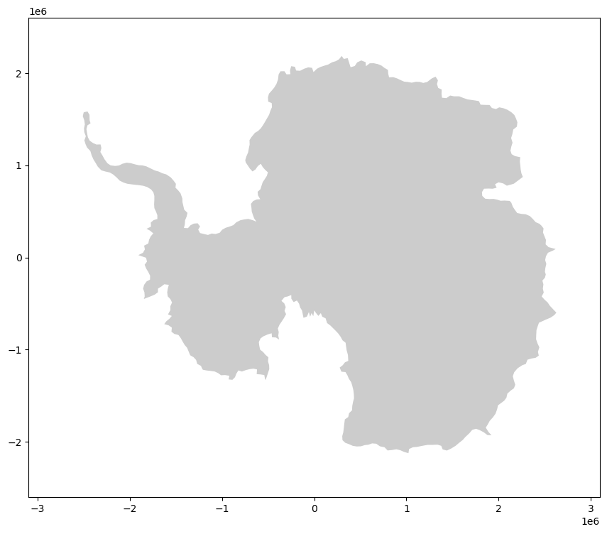
Stereographic projections are common for mapping in polar regions. A lot of legacy data products for both Greenland and Antarctica use polar stereographic projections. Some other polar products, such as NSIDC EASE/EASE-2 grids, are in equal-area projections.
Here, we’ll use the transform to get the latitude and longitude coordinates of points in this projection (an inverse tranformation), and get the polar stereographic coordinates for plotting a circle around the standard parallel (-71°) of this projection (a forward transformation).
The standard parallel of a stereographic projection is the latitude where there is no scale distortion.
def scale_factors(
        lat: np.ndarray,
        flat: float = 1.0/298.257223563,
        reference_latitude: float = 70.0,
        metric: str = 'area'
    ):
    """
    Calculates scaling factors to account for polar stereographic
    distortion including special case of at the exact pole

    Parameters
    ----------
    lat: np.ndarray
        latitude (degrees north)
    flat: float, default 1.0/298.257223563
        ellipsoidal flattening
    reference_latitude: float, default 70.0
        reference latitude (true scale latitude)
    metric: str, default 'area'
        metric to calculate scaling factors

            - ``'distance'``: scale factors for distance
            - ``'area'``: scale factors for area

    Returns
    -------
    scale: np.ndarray
        scaling factors at input latitudes
    """
    assert metric.lower() in ['distance', 'area'], 'Unknown metric'
    # convert latitude from degrees to positive radians
    theta = np.abs(lat)*np.pi/180.0
    # convert reference latitude from degrees to positive radians
    theta_ref = np.abs(reference_latitude)*np.pi/180.0
    # square of the eccentricity of the ellipsoid
    # ecc2 = (1-b**2/a**2) = 2.0*flat - flat^2
    ecc2 = 2.0*flat - flat**2
    # eccentricity of the ellipsoid
    ecc = np.sqrt(ecc2)
    # calculate ratio at input latitudes
    m = np.cos(theta)/np.sqrt(1.0 - ecc2*np.sin(theta)**2)
    t = np.tan(np.pi/4.0 - theta/2.0)/((1.0 - ecc*np.sin(theta)) / \
        (1.0 + ecc*np.sin(theta)))**(ecc/2.0)
    # calculate ratio at reference latitude
    mref = np.cos(theta_ref)/np.sqrt(1.0 - ecc2*np.sin(theta_ref)**2)
    tref = np.tan(np.pi/4.0 - theta_ref/2.0)/((1.0 - ecc*np.sin(theta_ref)) / \
        (1.0 + ecc*np.sin(theta_ref)))**(ecc/2.0)
    # distance scaling
    k = (mref/m)*(t/tref)
    kp = 0.5*mref*np.sqrt(((1.0+ecc)**(1.0+ecc))*((1.0-ecc)**(1.0-ecc)))/tref
    if (metric.lower() == 'distance'):
        # distance scaling
        scale = np.where(np.isclose(theta, np.pi/2.0), 1.0/kp, 1.0/k)
    elif (metric.lower() == 'area'):
        # area scaling
        scale = np.where(np.isclose(theta, np.pi/2.0), 1.0/(kp**2), 1.0/(k**2))
    return scale
crs4326 = pyproj.CRS.from_epsg(4326) # WGS84
crs3031 = pyproj.CRS.from_epsg(3031) # Antarctic Polar Stereographic
transformer = pyproj.Transformer.from_crs(crs4326, crs3031, always_xy=True)fig,ax3 = plt.subplots(num=3, figsize=(10,7.5))
xmin,xmax,ymin,ymax = (-3100000,3100000,-2600000,2600000)
dx,dy = (10000,10000)
# create a grid of polar stereographic points
X = np.arange(xmin,xmax+dx,dx)
Y = np.arange(ymin,ymax+dy,dy)
gridx,gridy = np.meshgrid(X, Y)
# convert polar stereographic points to latitude/longitude (WGS84)
gridlon,gridlat = transformer.transform(gridx, gridy,
direction=pyproj.enums.TransformDirection.INVERSE)
# calculate and plot grid area
cf = crs3031.to_cf()
flat = 1.0/cf['inverse_flattening']
sp = cf['standard_parallel']
gridarea = scale_factors(gridlat, flat=flat, reference_latitude=sp)
im = ax3.imshow(gridarea,
extent=(xmin,xmax,ymin,ymax),
interpolation='nearest',
cmap=plt.get_cmap('plasma'),
origin='lower')
# add circle around standard parallel
ref_lon = np.arange(360)
ref_lat = np.ones((360))*sp
# convert latitude/longitude (WGS84) points to polar stereographic
ref_x,ref_y = transformer.transform(ref_lon, ref_lat,
direction=pyproj.enums.TransformDirection.FORWARD)
l, = ax3.plot(ref_x, ref_y, '--', color='w', dashes=(8,4), label='Standard Parallel')
# add coastlines
world_antarctic.plot(ax=ax3, color='none', edgecolor='black')
# set x and y limits
ax3.set_xlim(xmin,xmax)
ax3.set_ylim(ymin,ymax)
ax3.set_aspect('equal', adjustable='box')
# add x and y labels
x_info,y_info = crs3031.axis_info
ax3.set_xlabel('{0} [{1}]'.format(x_info.name,x_info.unit_name))
ax3.set_ylabel('{0} [{1}]'.format(y_info.name,y_info.unit_name))
# add colorbar
cbar = plt.colorbar(im, cax=fig.add_axes([0.92, 0.08, 0.025, 0.90]))
cbar.ax.set_ylabel('Normalized Grid Area')
cbar.solids.set_rasterized(True)
# add legend
lgd = ax3.legend(loc=4,frameon=False)
lgd.get_frame().set_alpha(1.0)
for line in lgd.get_lines():
line.set_linewidth(6)
for i,text in enumerate(lgd.get_texts()):
text.set_color(l.get_color())
fig.subplots_adjust(left=0.06,right=0.9,bottom=0.08,top=0.98)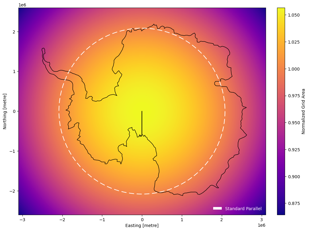
Why is there a black line to the pole? Because this coastline was reprojected from a Equirectangular projection. That’s the bottom of the Equirectangular map.
Reproject other data
Often you have other data or contextual information that you need to get into your data’s CRS to visualize.
For example, McMurdo Research Station is at (-77.846° S, 166.676° E). How to we plot this without using geopandas?
pyproj transform objects can be used to change the Coordinate Reference System of arrays
This will transform our latitude and longitude coordinates into coordinates in meters from the map origin
# convert location of McMurdo station to polar stereographic
McMurdo = (166.676, -77.846)
McMurdo_3031 = transformer.transform(*McMurdo)

fig, ax = plt.subplots()
world_antarctic.plot(ax=ax, color='0.8', edgecolor='none')
ax.plot(McMurdo_3031[0], McMurdo_3031[1], 'ro')
# set x and y limits
xmin,xmax,ymin,ymax = (-3100000,3100000,-2600000,2600000)
ax.set_xlim(xmin,xmax)
ax.set_ylim(ymin,ymax)
ax.set_aspect('equal', adjustable='box')
ax.set_title(f'McMurdo Station {McMurdo}');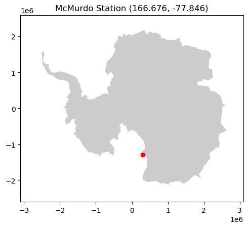
Reference Systems and Datums
Coordinates are defined to be in reference to the origins of the coordinate system
- Horizontally, coordinates are in reference to the Equator and the Prime Meridian
- Vertically, heights are in reference to a datum
Two common vertical datums are the reference ellipsoid and the reference geoid.
What are they and what is the difference?
- To first approximation, the Earth is a sphere (🐄) with a radius of 6371 kilometers.
- To a better approximation, the Earth is a slightly flattened ellipsoid with the polar axis 22 kilometers shorter than the equatorial axis.
- To an even better approximation, the Earth’s shape can be described using a reference geoid, which undulates 10s of meters above and below the reference ellipsoid. The difference in height between the ellipsoid and the geoid are known as geoid heights.
The geoid is an equipotential surface, perpendicular to the force of gravity at all points and with a constant geopotential. Reference ellipsoids and geoids are both created to largely coincide with mean sea level if the oceans were at rest.
An ellipsoid can be considered a simplification of a geoid.
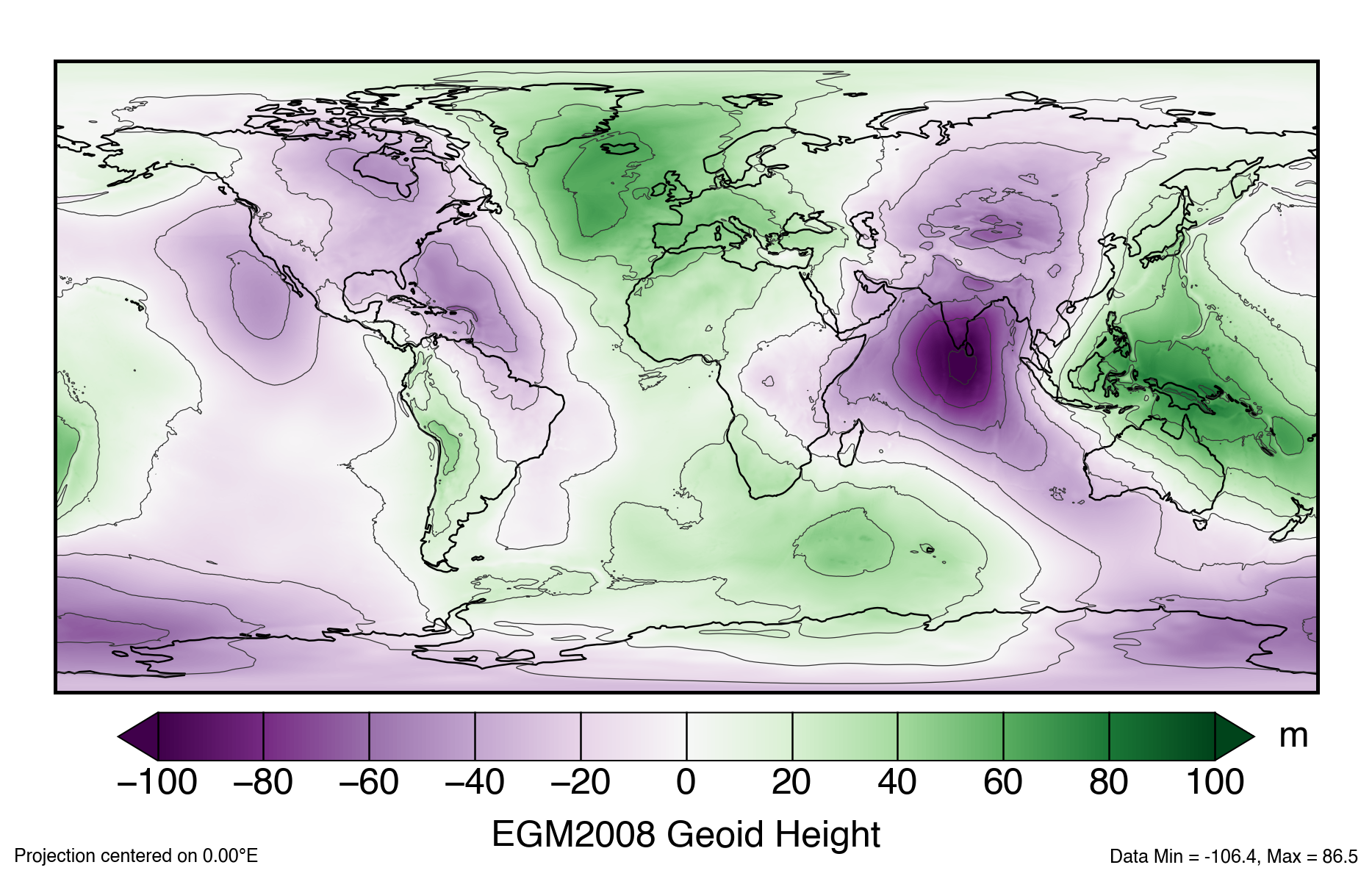
PROJ hosts grids for shifting both the horizontal and vertical datum, such as gridded EGM2008 geoid height values
Additional geoid height values can be calculated at the International Centre for Global Earth Models (ICGEM)
Vertically exaggerated, the Earth is sort of like a potato 🥔
Why Does This Matter?
ICESat-2 elevations are in reference to a specific version of the WGS84 ellipsoid. There are different “realizations” of the WGS84 ellipsoid. The accuracy of your positioning improves when the specific realization, rather than the ensemble, is used!
ICESat-2 data products also include geoid heights from the EGM2008 geoid. Different ground-based, airborne or satellite-derived elevations may use a separate datum entirely.
Different datums have different purposes. Heights above mean sea level are needed for ocean and sea ice heights, and are also commonly used for terrestrial mapping (e.g. as elevations of mountains). Ellipsoidal heights are commonly used for estimating land ice height change.
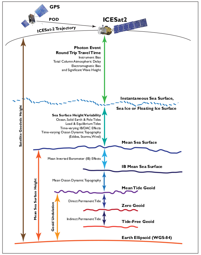
Modified from: Tapley, B. D. & M-C. Kim, Applications to Geodesy, Chapt. 10 in Satellite Altimetry and Earth Sciences, ed. by L-L. Fu & A. Cazenave, Academic Press, pp. 371-406, 2001.
Terrestrial Reference System
Locations of satellites are determined in an Earth-centered cartesian coordinate system
- X, Y, and Z measurements from the Earth’s center of mass
Up to Release-06, ICESat-2 has been set in the 2014 realization of the International Terrestrial Reference Frame (ITRF). For Release-07 onward, ICESat-2 will be set in the 2020 realization. Other satellite and airborne altimetry missions may be in a different ITRF entirely.
As opposed to simple vertical offsets, changing the terrestial reference system can involve both translation and rotation of the reference system. This involves converting from a geographic coordinate system into a Cartesian coordinate system.
Let’s visualize what the Cartesian coordinate system looks like:
def to_cartesian(lon,lat,h=0.0,a_axis=6378137.0,flat=1.0/298.257223563):
    """
    Converts geodetic coordinates to Cartesian coordinates

    Inputs:
        lon: longitude (degrees east)
        lat: latitude (degrees north)

    Options:
        h: height above ellipsoid (or sphere)
        a_axis: semimajor axis of the ellipsoid (default: WGS84)
            * for spherical coordinates set to radius of the Earth
        flat: ellipsoidal flattening (default: WGS84)
            * for spherical coordinates set to 0
    """
    # verify axes
    lon = np.atleast_1d(lon)
    lat = np.atleast_1d(lat)
    # fix coordinates to be 0:360
    lon[lon < 0] += 360.0
    # Linear eccentricity and first numerical eccentricity
    lin_ecc = np.sqrt((2.0*flat - flat**2)*a_axis**2)
    ecc1 = lin_ecc/a_axis
    # convert from geodetic latitude to geocentric latitude
    dtr = np.pi/180.0
    # geodetic latitude in radians
    latitude_geodetic_rad = lat*dtr
    # prime vertical radius of curvature
    N = a_axis/np.sqrt(1.0 - ecc1**2.0*np.sin(latitude_geodetic_rad)**2.0)
    # calculate X, Y and Z from geodetic latitude and longitude
    X = (N + h) * np.cos(latitude_geodetic_rad) * np.cos(lon*dtr)
    Y = (N + h) * np.cos(latitude_geodetic_rad) * np.sin(lon*dtr)
    Z = (N * (1.0 - ecc1**2.0) + h) * np.sin(latitude_geodetic_rad)
    # return the cartesian coordinates
    return (X,Y,Z)
fig,ax2 = plt.subplots(num=2, subplot_kw=dict(projection='3d'))
minlon,maxlon,minlat,maxlat = (-180,180,-90,90)
dlon,dlat = (10.0,10.0)
longitude = np.arange(minlon,maxlon+dlon,dlon)
latitude = np.arange(minlat,maxlat+dlat,dlat)
gridlon,gridlat = np.meshgrid(longitude, latitude)
height = np.zeros_like(gridlon)
X,Y,Z = to_cartesian(gridlon, gridlat, h=height)
ax2.scatter3D(X, Y, Z, c=gridlat)
plt.show()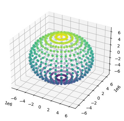
Yep, that looks like an ellipsoid
pyproj CRS Tricks
pyproj CRS objects can:
- Be converted to different methods of describing the CRS, such a to a
PROJstring or WKT
proj3031 = crs3031.to_proj4()
wkt3031 = crs3031.to_wkt()
assert(crs3031.is_exact_same(pyproj.CRS.from_wkt(wkt3031)))
print(proj3031)
+proj=stere +lat_0=-90 +lat_ts=-71 +lon_0=0 +x_0=0 +y_0=0 +datum=WGS84 +units=m +no_defs +type=crs
- Provide information about each coordinate reference system, such as the name, area of use and axes units.
for EPSG in (3031,3413,5936,6931,6932):
  crs = pyproj.CRS.from_epsg(EPSG)
  x_info,y_info = crs.axis_info
  print(f'{crs.name} ({EPSG})')
  print(f'\tRegion: {crs.area_of_use.name}')
  print(f'\tScope: {crs.scope}')
  print(f'\tAxes: {x_info.name} ({x_info.unit_name}), {y_info.name} ({y_info.unit_name})')
WGS 84 / Antarctic Polar Stereographic (3031)
Region: Antarctica.
Scope: Antarctic Digital Database and small scale topographic mapping.
Axes: Easting (metre), Northing (metre)
WGS 84 / NSIDC Sea Ice Polar Stereographic North (3413)
Region: Northern hemisphere - north of 60°N onshore and offshore, including Arctic.
Scope: Polar research.
Axes: Easting (metre), Northing (metre)
WGS 84 / EPSG Alaska Polar Stereographic (5936)
Region: Northern hemisphere - north of 60°N onshore and offshore, including Arctic.
Scope: Arctic small scale mapping - Alaska-centred.
Axes: Easting (metre), Northing (metre)
WGS 84 / NSIDC EASE-Grid 2.0 North (6931)
Region: Northern hemisphere.
Scope: Environmental science - used as basis for EASE grid.
Axes: Easting (metre), Northing (metre)
WGS 84 / NSIDC EASE-Grid 2.0 South (6932)
Region: Southern hemisphere.
Scope: Environmental science - used as basis for EASE grid.
Axes: Easting (metre), Northing (metre)
- Get coordinate reference system metadata for including in files
print('Climate and Forecast (CF) conventions')
cf = pyproj.CRS.from_epsg(5936).to_cf()
for key,val in cf.items():
    print(f'\t{key}: {val}')
Climate and Forecast (CF) conventions
crs_wkt: PROJCRS["WGS 84 / EPSG Alaska Polar Stereographic",BASEGEOGCRS["WGS 84",ENSEMBLE["World Geodetic System 1984 ensemble",MEMBER["World Geodetic System 1984 (Transit)"],MEMBER["World Geodetic System 1984 (G730)"],MEMBER["World Geodetic System 1984 (G873)"],MEMBER["World Geodetic System 1984 (G1150)"],MEMBER["World Geodetic System 1984 (G1674)"],MEMBER["World Geodetic System 1984 (G1762)"],MEMBER["World Geodetic System 1984 (G2139)"],MEMBER["World Geodetic System 1984 (G2296)"],ELLIPSOID["WGS 84",6378137,298.257223563,LENGTHUNIT["metre",1]],ENSEMBLEACCURACY[2.0]],PRIMEM["Greenwich",0,ANGLEUNIT["degree",0.0174532925199433]],ID["EPSG",4326]],CONVERSION["EPSG Alaska Polar Stereographic",METHOD["Polar Stereographic (variant A)",ID["EPSG",9810]],PARAMETER["Latitude of natural origin",90,ANGLEUNIT["degree",0.0174532925199433],ID["EPSG",8801]],PARAMETER["Longitude of natural origin",-150,ANGLEUNIT["degree",0.0174532925199433],ID["EPSG",8802]],PARAMETER["Scale factor at natural origin",0.994,SCALEUNIT["unity",1],ID["EPSG",8805]],PARAMETER["False easting",2000000,LENGTHUNIT["metre",1],ID["EPSG",8806]],PARAMETER["False northing",2000000,LENGTHUNIT["metre",1],ID["EPSG",8807]]],CS[Cartesian,2],AXIS["easting (X)",south,MERIDIAN[-60,ANGLEUNIT["degree",0.0174532925199433]],ORDER[1],LENGTHUNIT["metre",1]],AXIS["northing (Y)",south,MERIDIAN[30,ANGLEUNIT["degree",0.0174532925199433]],ORDER[2],LENGTHUNIT["metre",1]],USAGE[SCOPE["Arctic small scale mapping - Alaska-centred."],AREA["Northern hemisphere - north of 60°N onshore and offshore, including Arctic."],BBOX[60,-180,90,180]],ID["EPSG",5936]]
semi_major_axis: 6378137.0
semi_minor_axis: 6356752.314245179
inverse_flattening: 298.257223563
reference_ellipsoid_name: WGS 84
longitude_of_prime_meridian: 0.0
prime_meridian_name: Greenwich
geographic_crs_name: WGS 84
horizontal_datum_name: World Geodetic System 1984 ensemble
projected_crs_name: WGS 84 / EPSG Alaska Polar Stereographic
grid_mapping_name: polar_stereographic
latitude_of_projection_origin: 90.0
straight_vertical_longitude_from_pole: -150.0
false_easting: 2000000.0
false_northing: 2000000.0
scale_factor_at_projection_origin: 0.994
You can also manually create a pipeline to do coordinate reference systems conversions. These are like recipes for converting coordinate reference systems.
Remember converting latitude and longitude into cartesian coordinates? We can do that with a pipeline!
fig,ax2 = plt.subplots(num=2, subplot_kw=dict(projection='3d'))
minlon,maxlon,minlat,maxlat = (-180,180,-90,90)
dlon,dlat = (10.0,10.0)
longitude = np.arange(minlon,maxlon+dlon,dlon)
latitude = np.arange(minlat,maxlat+dlat,dlat)
gridlon,gridlat = np.meshgrid(longitude, latitude)
height = np.zeros_like(gridlon)
pipeline = """+proj=pipeline
    +step +proj=unitconvert +xy_in=deg +z_in=m +xy_out=rad +z_out=m
    +step +proj=cart +ellps=WGS84"""
transform = pyproj.Transformer.from_pipeline(pipeline)
X,Y,Z = transform.transform(gridlon,gridlat,height)
ax2.scatter3D(X,Y,Z, c=gridlat)
plt.show()
projinfo can list possible pipelines for converting between coordinate reference systems
Here is the pipeline PROJ chose to convert from latitude and longitude into polar stereographic
!projinfo -s EPSG:4326 -t EPSG:3031 -o PROJ --hide-ballpark --spatial-test intersectsCandidate operations found: 1
-------------------------------------
Operation No. 1:
EPSG:19992, Antarctic Polar Stereographic, 0 m, Antarctica.
PROJ string:
+proj=pipeline
+step +proj=axisswap +order=2,1
+step +proj=unitconvert +xy_in=deg +xy_out=rad
+step +proj=stere +lat_0=-90 +lat_ts=-71 +lon_0=0 +x_0=0 +y_0=0 +ellps=WGS84
Geospatial Data
What is Geospatial Data? Data that has location information associated with it.
Geospatial data comes in two flavors: vector and raster
- Vector data is composed of points, lines, and polygons
- Raster data is composed of individual grid cells
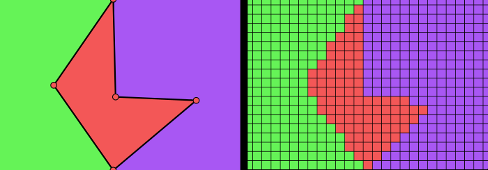
Vector vs. Raster from Planet
Vector data will provide geometric information for every point or vertex in the geometry.
Raster data will provide geometric information for a particular corner, which can be combined with the grid cell sizes and grid dimensions to get the grid cell coordinates.
Common vector file formats:
GeoJSONshapefileGeoPackage- ESRI
geodatabase kml/kmzgeoparquet
Common raster file formats:
GeoTIFF/cogjpegpng
File formats used for both:
netCDF4HDF5zarr
All geospatial data (raster and vector) should have metadata for extracting the coordinate reference system of the data. Some of this metadata is not included with the files but can be found in the documentation.
There are different tools for working with raster and vector data. Some are more advantageous for one data type over the other.
Let’s find the coordinate reference system of some data products using some common geospatial tools.
Geospatial Data Abstraction Library
The Geospatial Data Abstraction Library (GDAL/OGR) is a powerful piece of software.
It can read, write and query a wide variety of raster and vector geospatial data formats, transform the coordinate system of images, and manipulate other forms of geospatial data.
It is the backbone of a large suite of geospatial libraries and programs.
There are a number of wrapper libraries (e.g. rasterio, rioxarray, shapely, fiona) that provide more user-friendly interfaces with GDAL functionality.
Similar to pyproj CRS objects, GDAL SpatialReference functions can provide a lot of information about a particular Coordinate Reference System
With GDAL, we can access raster and vector data that are available over network-based file systems and virtual file systems
/vsicurl/: http/https/ftp files/vsis3/: AWS S3 files/vsigs/: Google Cloud Storage files/vsizip/: zip archives/vsitar/: tar/tgz archives/vsigzip/: gzipped files
These can be chained together to access compressed files over networks
Vector Data
We can use GDAL virtual file systems to access the intermediate resolution shapefile of the Global Self-consistent, Hierarchical, High-resolution Geography Database from its https server.
ogrinfo is a GDAL/OGR tool for inspecting vector data. We’ll get a summary (-so) of all data (-al) in read-only mode (-ro).
!ogrinfo -so -al -ro /vsizip//vsicurl/http://www.soest.hawaii.edu/pwessel/gshhg/gshhg-shp-2.3.7.zip/GSHHS_shp/i/GSHHS_i_L1.shpINFO: Open of `/vsizip//vsicurl/http://www.soest.hawaii.edu/pwessel/gshhg/gshhg-shp-2.3.7.zip/GSHHS_shp/i/GSHHS_i_L1.shp'
using driver `ESRI Shapefile' successful.
Layer name: GSHHS_i_L1
Metadata:
DBF_DATE_LAST_UPDATE=2017-06-15
Geometry: Polygon
Feature Count: 32830
Extent: (-180.000000, -68.919814) - (180.000000, 83.633389)
Layer SRS WKT:
GEOGCRS["WGS 84",
    DATUM["World Geodetic System 1984",
        ELLIPSOID["WGS 84",6378137,298.257223563,
            LENGTHUNIT["metre",1]]],
    PRIMEM["Greenwich",0,
        ANGLEUNIT["degree",0.0174532925199433]],
    CS[ellipsoidal,2],
        AXIS["latitude",north,
            ORDER[1],
            ANGLEUNIT["degree",0.0174532925199433]],
        AXIS["longitude",east,
            ORDER[2],
            ANGLEUNIT["degree",0.0174532925199433]],
    ID["EPSG",4326]]
Data axis to CRS axis mapping: 2,1
id: String (80.0)
level: Integer (9.0)
source: String (80.0)
parent_id: Integer (9.0)
sibling_id: Integer (9.0)
area: Real (24.15)
Reading Vector Data
gshhg_i = gpd.read_file('/vsizip//vsicurl/http://www.soest.hawaii.edu/pwessel/gshhg/gshhg-shp-2.3.7.zip/GSHHS_shp/i/GSHHS_i_L1.shp')
print(gshhg_i.crs)
EPSG:4326
Let’s use these coastlines to make a plot of Greenland in a Polar Stereographic projection (EPSG:3413)
fig,ax4 = plt.subplots(num=4, figsize=(9,9))
crs3413 = pyproj.CRS.from_epsg(3413)
xmin,xmax,ymin,ymax = (-1530000, 1610000,-3600000, -280000)
# add coastlines
gshhg_i.to_crs(crs3413).plot(ax=ax4, color='0.8', edgecolor='none')
# set x and y limits
ax4.set_xlim(xmin,xmax)
ax4.set_ylim(ymin,ymax)
ax4.set_aspect('equal', adjustable='box')
# add x and y labels
x_info,y_info = crs3413.axis_info
ax4.set_xlabel('{0} [{1}]'.format(x_info.name,x_info.unit_name))
ax4.set_ylabel('{0} [{1}]'.format(y_info.name,y_info.unit_name))
# adjust subplot and show
fig.subplots_adjust(left=0.06,right=0.98,bottom=0.08,top=0.98)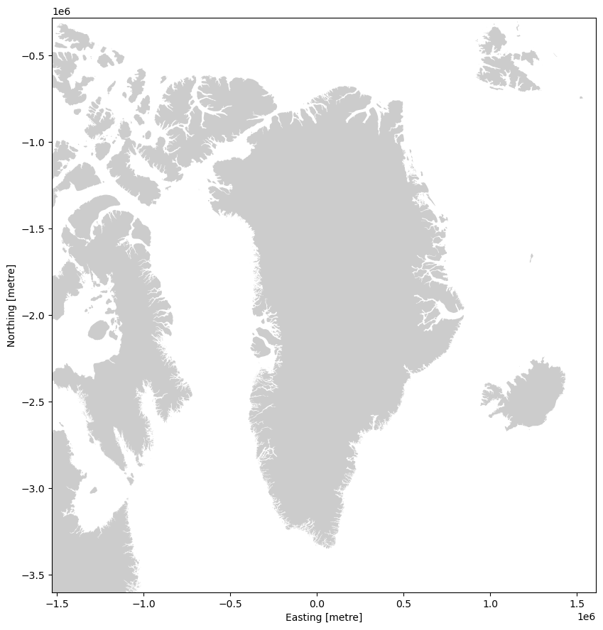
Even with intermediate resolution, we can add much better coastlines than the ones that ship with geodatasets!
All coastline resolutions available:
c: coarsel: lowi: intermediateh: highf: full
Raster Data
The same virtual file system commands can be used with raster images.
Let’s inspect some elevation data from the COP3 DEM.
gdalinfo allows us to inspect the format, size, geolocation and Coordinate Reference System of raster imagery. Appending the -proj4 option will additionally output the PROJ string associated with this geotiff image.
! gdalinfo -proj4 "https://opentopography.s3.sdsc.edu/raster/COP30/COP30_hh/Copernicus_DSM_10_N47_00_W123_00_DEM.tif"Driver: GTiff/GeoTIFF
Files: none associated
Size is 3601, 3601
Coordinate System is:
GEOGCRS["WGS 84",
ENSEMBLE["World Geodetic System 1984 ensemble",
MEMBER["World Geodetic System 1984 (Transit)"],
MEMBER["World Geodetic System 1984 (G730)"],
MEMBER["World Geodetic System 1984 (G873)"],
MEMBER["World Geodetic System 1984 (G1150)"],
MEMBER["World Geodetic System 1984 (G1674)"],
MEMBER["World Geodetic System 1984 (G1762)"],
MEMBER["World Geodetic System 1984 (G2139)"],
MEMBER["World Geodetic System 1984 (G2296)"],
ELLIPSOID["WGS 84",6378137,298.257223563,
LENGTHUNIT["metre",1]],
ENSEMBLEACCURACY[2.0]],
PRIMEM["Greenwich",0,
ANGLEUNIT["degree",0.0174532925199433]],
CS[ellipsoidal,2],
AXIS["geodetic latitude (Lat)",north,
ORDER[1],
ANGLEUNIT["degree",0.0174532925199433]],
AXIS["geodetic longitude (Lon)",east,
ORDER[2],
ANGLEUNIT["degree",0.0174532925199433]],
USAGE[
SCOPE["Horizontal component of 3D system."],
AREA["World."],
BBOX[-90,-180,90,180]],
ID["EPSG",4326]]
Data axis to CRS axis mapping: 2,1
PROJ.4 string is:
'+proj=longlat +datum=WGS84 +no_defs'
Origin = (-123.000138888888884,48.000138888888891)
Pixel Size = (0.000277777777778,-0.000277777777778)
Metadata:
AREA_OR_POINT=Point
Image Structure Metadata:
LAYOUT=COG
COMPRESSION=DEFLATE
INTERLEAVE=BAND
Corner Coordinates:
Upper Left (-123.0001389, 48.0001389) (123d 0' 0.50"W, 48d 0' 0.50"N)
Lower Left (-123.0001389, 46.9998611) (123d 0' 0.50"W, 46d59'59.50"N)
Upper Right (-121.9998611, 48.0001389) (121d59'59.50"W, 48d 0' 0.50"N)
Lower Right (-121.9998611, 46.9998611) (121d59'59.50"W, 46d59'59.50"N)
Center (-122.5000000, 47.5000000) (122d30' 0.00"W, 47d30' 0.00"N)
Band 1 Block=512x512 Type=Float32, ColorInterp=Gray
Overviews: 1801x1801, 901x901, 451x451
Unit Type: metre
Reading Raster Data
We can read geotiff files using rasterio, which is a wrapper of GDAL for reading raster data
url = "https://opentopography.s3.sdsc.edu/raster/COP30/COP30_hh/Copernicus_DSM_10_N47_00_W123_00_DEM.tif"
ds = rioxarray.open_rasterio(url, masked=True).isel(band=0)
ds# plot location of DEM
fig,ax1 = plt.subplots(num=1, figsize=(10.375,5.0))
minlon,maxlon,minlat,maxlat = (-180,180,-90,90)
# add geometry of image
xmin, ymin, xmax, ymax = ds.rio.transform_bounds('EPSG:4326')
box = gpd.GeoSeries(shapely.geometry.box(xmin, ymin, xmax, ymax))
box.plot(ax=ax1,facecolor='red',edgecolor='red',alpha=0.5)
# add annotation
ax1.annotate("Here!", xy=(xmin,ymin), xytext=(xmin-15.0, ymin-15.0),
arrowprops=dict(arrowstyle="->",connectionstyle="arc3,rad=0.3",color='red'),
bbox=dict(boxstyle="square", fc="w", ec="w", pad=0.1),
color='red', weight='bold', xycoords='data', ha='center')
# add GSHHG coastlines
gshhg_i.plot(ax=ax1, color='none', edgecolor='black')
# set x and y limits
ax1.set_xlim(minlon,maxlon)
ax1.set_ylim(minlat,maxlat)
ax1.set_aspect('equal', adjustable='box')
# add x and y labels
ax1.set_xlabel('Longitude')
ax1.set_ylabel('Latitude')
# adjust subplot and show
fig.subplots_adjust(left=0.06,right=0.98,bottom=0.08,top=0.98)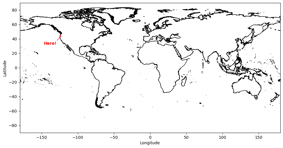
Okay! It covers Seattle and the University of Washington.
Let’s see what the DEM looks like for this granule
# create figure axis
fig, ax = plt.subplots(num=5)
im = ds.plot.imshow(ax=ax, interpolation='nearest',
    vmin=ds.values.min(), vmax=ds.values.max(),
    cmap=plt.cm.gray_r)
x,y = (-122.3117, 47.6533)
ax.plot(x, y, 'r*')
# add annotation
ax.annotate("UW eScience!", xy=(x,y-0.005), xytext=(x-0.1, y-0.1),
    arrowprops=dict(arrowstyle="->",connectionstyle="arc3,rad=0.3",color='red'),
    color='red', weight='bold', xycoords='data', ha='center')
# turn of frame and ticks
ax.set_frame_on(False)
ax.set_xticks([])
ax.set_yticks([])
plt.axis('off')
# adjust subplot within figure
fig.subplots_adjust(left=0, bottom=0, right=1, top=1, wspace=None, hspace=None)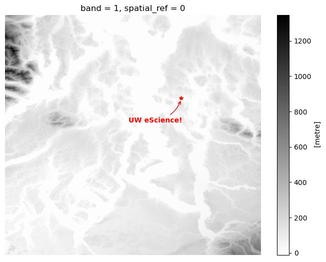
Warping Raster Imagery
Warping transfers a raster image from one Coordinate Reference System (CRS) into another.
We can use GDAL to reproject the imagery data into another CRS or change the pixel resolution of the raster image.
Ground control points (GCPs) can also be applied to georeference raw maps or imagery.
Raster Georeferencing from ESRI
Rasterio Transforms
For every rasterio object, there is an associated affine transform (ds.transform), which allows you to transfer from image coordinates to geospatial coordinates.
Affine Transformation: maps between pixel locations in (row, col) coordinates to (x, y) spatial positions:
x,y = ds.transform*(row,col)
Upper left coordinate:
row = 0col = 0
Lower right coordinate:
row = ds.widthcol = ds.height
Raster Georeferencing from ESRI
rioxarray does these affine transformations under the hood when reprojecting images. We can use these tools to warp our raster image into a lower resolution.
# degrade resolution from 1 arcsecond to 8 arcseconds
dst_res = 8.0/3600.0
warped = ds.rio.reproject(crs4326, resolution=(dst_res,dst_res))

# plot warped DEM
fig,ax1 = plt.subplots(num=1, figsize=(10.375,5.0))
# add geometry of image
im = warped.plot.imshow(ax=ax1, interpolation='nearest',
    vmin=ds.values.min(), vmax=ds.values.max(),
    cmap=plt.cm.gray_r)
# add coastlines
gshhg_i.plot(ax=ax1, color='none', edgecolor='black')
# set x and y limits
ax1.set_xlim(warped.x.min(), warped.x.max())
ax1.set_ylim(warped.y.min(), warped.y.max())
ax1.set_aspect('equal', adjustable='box')
# add x and y labels
ax1.set_xlabel('Longitude')
ax1.set_ylabel('Latitude')
# adjust subplot and show
fig.subplots_adjust(left=0.06,right=0.98,bottom=0.08,top=0.98)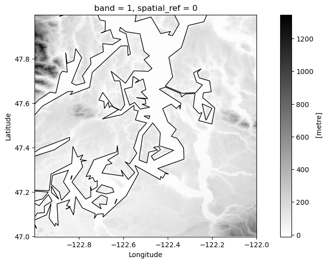
Saving Raster Data with rioxarray
# write an array as a raster band
# copernicus DEM naming convention for spacing:
# 03: 0.3-arcsecond grid, 04: 0.4-arcsecond grid, 10: 1-arcsecond grid, 30: 3-arcsecond grid
warped.rio.to_raster('Copernicus_DSM_80_N47_00_W123_00_DEM.tif', driver='cog')
Applying Concepts: ICESat-2
Let’s take what we just learned and apply it to ICESat-2
We’ll download a granule of ICESat-2 ATL06 land ice heights from the National Snow and Ice Data Center (NSIDC). ATL06 is along-track data stored in an HDF5 file with geospatial coordinates latitude and longtude (WGS84). Within an ATL06 file, there are six beam groups (gt1l, gt1r, gt2l, gt2r, gt3l, gt3r) that correspond to the orientation of the beams on the ground.
def build_granule_name(short_name, track, cycle, hemisphere=None, granule=None):
    # repeat ground track (RGT)
    tttt = str(track).zfill(4)
    # orbital cycle
    cc = str(cycle).zfill(2)
    # ice hemisphere flag (01=north, 02=south)
    hh = str(hemisphere).zfill(2) if hemisphere is not None else "??"
    # granule number (ranges from 1-14, always 01 for atmosphere products)
    nn = str(granule).zfill(2) if granule is not None else "??"
    # patterns vary by product
    along_track_products = ("ATL03", "ATL04", "ATL06", "ATL08",
        "ATL09", "ATL10", "ATL12", "ATL13", "ATL16", "ATL17",
        "ATL19", "ATL22", "ATL24")
    sea_ice_products = ("ATL07", "ATL10", "ATL20", "ATL21")
    # use single character wildcards "?" for any unset parameters
    if short_name in sea_ice_products:
        return f"{short_name}-{hh}_{14 * '?'}_{tttt}{cc}??_*"
    elif short_name in along_track_products:
        return f"{short_name}_{14 * '?'}_{tttt}{cc}{nn}_*"
# build credentials for accessing ICESat-2 data
auth = earthaccess.login(strategy="environment")
# query CMR for ATL06 files
pattern = build_granule_name(short_name="ATL06", track=9, cycle=14, granule=12)
granules = earthaccess.search_data(
short_name="ATL06",
granule_name=pattern,
)
granules[0]# download or stream ATL06 granules
if (AWS_DEFAULT_REGION == 'us-west-2'):
buffers = earthaccess.open(granules)
else:
buffers = earthaccess.download(granules, local_path='.')
# read multiple HDF5 groups and merge into a dataset
groups = ['gt1l/land_ice_segments', 'gt1l/land_ice_segments/dem']
ds = xr.merge([xr.open_dataset(buffers[0], group=g) for g in groups])
# inspect ATL06 data for beam group
dsxarray has a handy to_dataframe function to convert to pandas
# For simplicity take first 500 high-quality points into a Geopandas Geodataframe
df = ds.where(ds.atl06_quality_summary==0).isel(delta_time=slice(0,500)).to_dataframe()
gdf = gpd.GeoDataFrame(df, geometry=gpd.points_from_xy(df.longitude, df.latitude), crs='epsg:7661')
gdf.head()use explore to create an interactive map of our ICESat-2 points
gdf.explore(column='h_li')Copernicus DEM
Let’s compare ICESat-2 elevations against a public, gridded global digital elevation model (DEM), the Copernicus DEM. This DEM is with respect to the EGM2008 geoid, and so we’ll have to convert our ICESat-2 points to be comparable.
Just as Geopandas adds CRS-aware capabilities to Dataframes, RioXarray adds CRS-aware functions to XArray multidimensional arrays (e.g. sets of images).
COP30 = rioxarray.open_rasterio('https://opentopography.s3.sdsc.edu/raster/COP30/COP30_hh.vrt', chunks=True)
# Crop by Bounding box of all the ATL06 points
minx, miny, maxx, maxy = gdf.total_bounds
COP30 = COP30.rio.clip_box(minx, miny, maxx, maxy).sel(band=1)
COP30Convert ATL06 Ellipsoidal Heights to Orthometric
Check out the ICESat-2 User Comparison Guide for more info
gdf['h_ortho'] = gdf.h_li - (gdf.geoid_h + gdf.geoid_free2mean)
# calculate elevation difference between ATL06 and COP30
x = xr.DataArray(gdf.geometry.x.values, dims='z')
y = xr.DataArray(gdf.geometry.y.values, dims='z')
gdf['dh'] = gdf.h_ortho - COP30.sel(x=x, y=y, method='nearest')
Compare COP30 DEM with ATL06
fig, ax = plt.subplots(ncols=3, sharex=True, sharey=True)
cmap1 = plt.get_cmap('viridis')
cmap2 = plt.get_cmap('coolwarm')
vmin = np.minimum(COP30.min().values, gdf.h_ortho.min())
vmax = np.maximum(COP30.max().values, gdf.h_ortho.max())
COP30.plot.imshow(ax=ax[0], cmap=cmap1, vmin=vmin, vmax=vmax, add_labels=False, add_colorbar=False)
gdf.plot(column="h_ortho", ax=ax[1], cmap=cmap1, vmin=vmin, vmax=vmax, markersize=1, legend=True)
gdf.plot(column="dh", ax=ax[2], cmap=cmap2, norm=mcolors.CenteredNorm(), markersize=1, legend=True)
fig.tight_layout()
plt.show()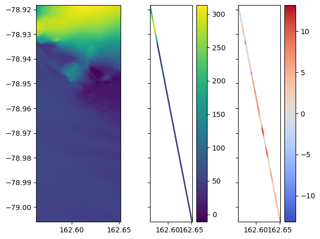
Resources
There is a lot of great educational material to learn more about these topics. We recommend checking out:
- Robbins, J., Sutterley, T., Neumann, T., Kurtz, N., Bagnardi, M., Brunt, K., Gibbons, A., Hancock, D., Lee, J., & Luthcke, S. (2025). ICESat-2 Data Comparison User’s Guide. 10.5281/ZENODO.16389970