USACE topobathy vis with Google Earth Engine
Computing environment
We’ll be using the following Python libraries in this notebook:
%matplotlib widget
import ee
import geemap
---------------------------------------------------------------------------
ModuleNotFoundError                       Traceback (most recent call last)
Input In [1], in <cell line: 1>()
----> 1 get_ipython().run_line_magic('matplotlib', 'widget')
      2 import ee
      3 import geemap

File /opt/hostedtoolcache/Python/3.9.12/x64/lib/python3.9/site-packages/IPython/core/interactiveshell.py:2294, in InteractiveShell.run_line_magic(self, magic_name, line, _stack_depth)
   2292     kwargs['local_ns'] = self.get_local_scope(stack_depth)
   2293 with self.builtin_trap:
-> 2294     result = fn(*args, **kwargs)
   2295 return result

File /opt/hostedtoolcache/Python/3.9.12/x64/lib/python3.9/site-packages/IPython/core/magics/pylab.py:99, in PylabMagics.matplotlib(self, line)
     97     print("Available matplotlib backends: %s" % backends_list)
     98 else:
---> 99     gui, backend = self.shell.enable_matplotlib(args.gui.lower() if isinstance(args.gui, str) else args.gui)
    100     self._show_matplotlib_backend(args.gui, backend)

File /opt/hostedtoolcache/Python/3.9.12/x64/lib/python3.9/site-packages/IPython/core/interactiveshell.py:3444, in InteractiveShell.enable_matplotlib(self, gui)
   3423 def enable_matplotlib(self, gui=None):
   3424     """Enable interactive matplotlib and inline figure support.
   3425
   3426     This takes the following steps:
   (...)
   3442         display figures inline.
   3443     """
-> 3444     from matplotlib_inline.backend_inline import configure_inline_support
   3446     from IPython.core import pylabtools as pt
   3447     gui, backend = pt.find_gui_and_backend(gui, self.pylab_gui_select)

File /opt/hostedtoolcache/Python/3.9.12/x64/lib/python3.9/site-packages/matplotlib_inline/backend_inline.py:6, in <module>
      1 """A matplotlib backend for publishing figures via display_data"""
      3 # Copyright (c) IPython Development Team.
      4 # Distributed under the terms of the BSD 3-Clause License.
----> 6 import matplotlib
      7 from matplotlib.backends.backend_agg import (  # noqa
      8     new_figure_manager,
      9     FigureCanvasAgg,
     10     new_figure_manager_given_figure,
     11 )
     12 from matplotlib import colors

ModuleNotFoundError: No module named 'matplotlib'
import sys
sys.path.append('../')
from coastal.gis import dist_latlon2meters
from coastal.plot import plot_from_oa_url
Google Earth Engine Authentication and Initialization
GEE requires you to authenticate your access, so if ee.Initialize() does not work you first need to run ee.Authenticate(). This gives you a link at which you can use your google account that is associated with GEE to get an authorization code. Copy the authorization code into the input field and hit enter to complete authentication.
try:
    ee.Initialize()
except:
    ee.Authenticate()
    ee.Initialize()
Visualize USACE Topobathy data for Alaska
Data are from https://chs.coast.noaa.gov/htdata/raster2/elevation/ and are stored as an imageCollection here
topobathyColl = ee.ImageCollection('projects/uaf-coastal-mapping/assets/USACE_AK_DEM')
print('Number of DEMs in the collection (all of AK 2019): ', topobathyColl.size().getInfo())
Number of DEMs in the collection (all of AK 2019): 1147
Interactive map to visualize the entire collection. You can zoom around and see where the USACE collected data in western Alaska in 2019.
# initiate our map object with geemap
Map = geemap.Map()
Map.setCenter(-163.0222151036337, 64.58021590637386, zoom=7);
# Add a satellite basemap
Map.add_basemap('SATELLITE')
Map.layer_opacity(name='Google Satellite', value=0.8)
# Define our visualization parameters for the DEM collection
vis = {
    'min': -4,
    'max': 100,
    'palette': ['440154', '433982', '30678D', '218F8B', '36B677', '8ED542', 'FDE725'], # viridis color palette because I like it :)
}
Map.addLayer(topobathyColl, vis, 'Topobathy')
Map.add_minimap(zoom=3)

Map
Select by geographic region of interest
# Specify region of interest from geojson file
fn = 'data/whitemountain.geojson' # a geojson for white mountain, AK. You could also use a shapefile, etc.
aoi = geemap.geojson_to_ee(fn)
whiteMtn = topobathyColl.filterBounds(aoi)
print('Number of White Mountain area DEMs: ', whiteMtn.size().getInfo())

# access other collection details with .getInfo (note this can take a while).
Number of White Mountain area DEMs: 456
# initiate our map object with geemap
Map = geemap.Map()
Map.setCenter(-163.0222151036337, 64.58021590637386, zoom=8);
# Add a satellite basemap
Map.add_basemap('SATELLITE')
Map.layer_opacity(name='Google Satellite', value=0.8)
# Define our visualization parameters for the DEM collection
vis = {
    'min': -4,
    'max': 130,
    'palette': ['440154', '433982', '30678D', '218F8B', '36B677', '8ED542', 'FDE725'], # viridis color palette because I like it :)
}
Map.addLayer(whiteMtn, vis, 'Topobathy')
Map.addLayer(aoi, {}, 'White Mountain, AK')
Map.layer_opacity(name='White Mountain, AK', value=0.6)
Map.add_minimap(zoom=3)

Map
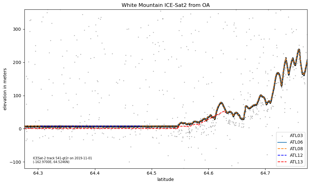
Overlay with example IS2 track:
with OpenAltimetry
%%capture
# get data from OpenAltimetry (following DataVis tutorial)
url = 'http://openaltimetry.org/data/api/icesat2/atl06?date=2019-11-01&minx=-163.22047900505012&miny=64.27523261959732&maxx=-162.71950245931393&maxy=64.77401189132661&trackId=541&beamName=gt3r&beamName=gt3l&beamName=gt2r&beamName=gt2l&beamName=gt1r&beamName=gt1l&outputFormat=json'
gtx = 'gt2r'
myplot, mydata = plot_from_oa_url(url=url, gtx=gtx, title='White Mountain ICE-Sat2 from OA')
myplot.savefig('white_mountain_2019-11-01.jpg', dpi=300)
myplot
Ground Track Stats & Map
lat1, lat2 = mydata.atl08.lat[0], mydata.atl08.lat.iloc[-1]
lon1, lon2 = mydata.atl08.lon[0], mydata.atl08.lon.iloc[-1]

ground_track_length = dist_latlon2meters(lat1, lon1, lat2, lon2)
print('The ground track is about %.1f kilometers long.' % (ground_track_length/1e3))
The ground track is about 55.7 kilometers long.
Now we need to add our ICESat-2 gound track to that map. Let’s use the lon/lat coordinates of the ATL08 data product for this.
We also need to specify which Coordinate Reference System (CRS) our data is in. The longitude/latitude system that we are all quite familiar with is referenced by EPSG:4326. To add the ground track to the map we need to turn it into an Earth Engine “Feature Collection”.
ground_track_coordinates = list(zip(mydata.atl08.lon, mydata.atl08.lat))
ground_track_projection = 'EPSG:4326' # <-- this specifies that our data longitude/latitude in degrees [https://epsg.io/4326]
gtx_feature = ee.FeatureCollection(ee.Geometry.LineString(coords=ground_track_coordinates,
                                      proj=ground_track_projection,
                                      geodesic=True))
# gtx_feature # check that it is a feature collection for GEE
# overlay the track on our map.
Map.addLayer(gtx_feature, {'color': 'red'}, 'ground track')
Map