ICESat-2 ATL03 SlideRule Demo
Plot ATL03 data with different classifications over a region
ATL08 Land and Vegetation Height product photon classification
Experimental YAPC (Yet Another Photon Classification) photon-density-based classification
#
import numpy as np
import matplotlib.pyplot as plt
from sliderule import sliderule
from sliderule import icesat2
import ipyleaflet
import icepyx as ipx
from ipyleaflet import Map, GeoData, LayersControl,Rectangle, basemaps, basemap_to_tiles, TileLayer, SplitMapControl, Polygon
---------------------------------------------------------------------------
ModuleNotFoundError Traceback (most recent call last)
Input In [2], in <cell line: 1>()
----> 1 import numpy as np
2 import matplotlib.pyplot as plt
3 from sliderule import sliderule
ModuleNotFoundError: No module named 'numpy'
import sys
sys.path.append('../')
from coastal.beam import reduce_dataframe
from coastal.plot import plot_atl08, plot_yapc
url = "icesat2sliderule.org"
icesat2.init(url, verbose=False)
asset = "nsidc-s3"
Set-up the region info
# Specifying the necessary icepyx parameters
spatial_extent = [{'lat': 19.628873000, 'lon': -156.004160000},
{'lat': 19.641079616, 'lon': -156.004160000},
{'lat': 19.641079616, 'lon': -155.988668873},
{'lat': 19.628873000, 'lon': -155.988668873},
{'lat': 19.628873000, 'lon': -156.004160000}]
# icepx will want a bounding box with LL lon/lat, UR lon/lat
bb = [spatial_extent[0]['lon'], spatial_extent[0]['lat'],
spatial_extent[2]['lon'], spatial_extent[2]['lat']]
polygon = Polygon(
locations=spatial_extent,
color="green"
)
time_start = '2018-11-14'
time_end = '2020-11-15'
date_range = [time_start, time_end]
Visualize the region
First example uses ipyleflet and second uses icepx.
center = [spatial_extent[0]['lat'], spatial_extent[0]['lon']]
zoom = 14
m = Map(basemap=basemaps.Esri.WorldImagery, center=center, zoom=zoom)
m.add_layer(polygon);
m
You can also show the region with icepyx but then adding on layers is harder.
# Setup the icepx Query object
region = ipx.Query('ATL03', bb, date_range)
# Note this will fail if there are no data for the region and dates
# Visualize the region with icepx
region.visualize_spatial_extent()


Use SlideRule to retrieve ATL03 elevations with ATL08 classifications
This returns gdf a geodataframe. I had to change the version to 004 and futz with the dates and release to get some data.
%%time
# build sliderule parameters for ATL03 subsetting request
# SRT_LAND = 0
# SRT_OCEAN = 1
# SRT_SEA_ICE = 2
# SRT_LAND_ICE = 3
# SRT_INLAND_WATER = 4
parms = {
# processing parameters
"srt": icesat2.SRT_LAND,
"len": 20,
# classification and checks
# still return photon segments that fail checks
"pass_invalid": True,
# all photons
"cnf": -2,
# all land classification flags
"atl08_class": ["atl08_noise", "atl08_ground", "atl08_canopy", "atl08_top_of_canopy", "atl08_unclassified"],
# all photons
"yapc": dict(knn=0, win_h=6, win_x=11, min_ph=4, score=0),
}
# ICESat-2 data release; I futzed with this
release = '004'
# time bounds defined at top
# find granule for each region of interest
granules_list = icesat2.cmr(
version=release,
polygon=spatial_extent,
time_start=time_start,
time_end=time_end)
# create an empty geodataframe
parms["poly"] = spatial_extent
gdf = icesat2.atl03sp(
parms,
asset=asset,
version=release,
resources=granules_list)
CPU times: user 784 ms, sys: 56.6 ms, total: 841 ms
Wall time: 2.83 s
gdf.head()
| sc_orient | track | segment_dist | cycle | rgt | segment_id | delta_time | atl08_class | yapc_score | quality_ph | distance | height | atl03_cnf | pair | geometry | |
|---|---|---|---|---|---|---|---|---|---|---|---|---|---|---|---|
| time | |||||||||||||||
| 2018-12-30 22:13:36.723056352 | 0 | 3 | 2.181795e+06 | 2 | 38 | 108784 | 3.144322e+07 | 4 | 0 | 0 | -6.147984 | 605.831848 | -1 | 0 | POINT (-156.00028 19.62886) |
| 2018-12-30 22:13:36.723056352 | 0 | 3 | 2.181795e+06 | 2 | 38 | 108784 | 3.144322e+07 | 4 | 45 | 0 | -2.438688 | 568.637207 | -1 | 0 | POINT (-156.00028 19.62890) |
| 2018-12-30 22:13:36.723056352 | 0 | 3 | 2.181795e+06 | 2 | 38 | 108784 | 3.144322e+07 | 4 | 6 | 0 | -0.781777 | 552.024109 | -1 | 0 | POINT (-156.00028 19.62891) |
| 2018-12-30 22:13:36.723156356 | 0 | 3 | 2.181795e+06 | 2 | 38 | 108784 | 3.144322e+07 | 4 | 50 | 0 | -4.888332 | 600.334778 | -1 | 0 | POINT (-156.00028 19.62887) |
| 2018-12-30 22:13:36.723156356 | 0 | 3 | 2.181795e+06 | 2 | 38 | 108784 | 3.144322e+07 | 4 | 0 | 0 | -0.698229 | 558.321777 | -1 | 0 | POINT (-156.00028 19.62891) |
gdf.shape
(40049, 15)
Add the data to our region map
center = [spatial_extent[0]['lat'], spatial_extent[0]['lon']]
zoom = 14
m2 = Map(basemap=basemaps.Esri.WorldImagery, center=center, zoom=zoom)
m2.add_layer(polygon);
geo_data = GeoData(geo_dataframe = gdf.sample(n=1000, replace=False, random_state=1),
# style={'color': 'red', 'radius':1, 'fillColor': '#3366cc', 'opacity':0.5, 'weight':1.9, 'dashArray':'2', 'fillOpacity':0.6},
style={'color': 'red', 'radius':1},
# hover_style={'fillColor': 'red' , 'fillOpacity': 0.2},
# point_style={'radius': 1, 'color': 'red', 'fillOpacity': 0.8, 'fillColor': 'blue', 'weight': 3},
point_style={'radius': 1, 'color': 'red', 'fillOpacity': 0.8},
name = 'Release')
m2.add_layer(geo_data)
m2
Reduce GeoDataFrame to plot a single beam
This function is goint to subset the geodataframe. Since we had a span of dates, there are multiple dates (and beams). This function will also set the CRS (map projection).
See the function reduce_dataframe in ./coastal/beam.py.
Now we can subset our dataframe. First let’s see what is in it.
print('cycle', gdf['cycle'].unique())
print('track', gdf['track'].unique())
print('rgt', gdf['rgt'].unique())
print('rgt', gdf['rgt'].unique())
cycle [2 5 7]
track [3 2]
rgt [38]
rgt [38]
We want to select a single cycle, track and rgt. I tried cycle=2 and discovered that it was all unclassified, so I set cycle=5.
beam_type = 'strong'
project_srs = "EPSG:26912+EPSG:5703"
D3 = reduce_dataframe(gdf, cycle=5, rgt=38, track=3, beam='strong', crs=project_srs)
D3["atl08_class"].value_counts()
1 2523
0 569
2 292
3 126
4 73
Name: atl08_class, dtype: int64
Inspect Coordinate Reference System
D3.crs
<Compound CRS: EPSG:26912+EPSG:5703>
Name: NAD83 / UTM zone 12N + NAVD88 height
Axis Info [cartesian|vertical]:
- E[east]: Easting (metre)
- N[north]: Northing (metre)
- H[up]: Gravity-related height (metre)
Area of Use:
- undefined
Datum: North American Datum 1983
- Ellipsoid: GRS 1980
- Prime Meridian: Greenwich
Sub CRS:
- NAD83 / UTM zone 12N
- NAVD88 height
Plot the ATL08 classifications
First I will create a function to help with the plotting. See the function plot_atl08 in ./coastal/plot.py. The function returns the figure and plots it so use fig = plot_atl08(D3) or put a semicolon at the end.
plot_atl08(D3);
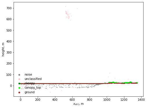
That doesn’t look so good. Let’s get rid of the pink (unclassified) dots. This looks better.
# Class 0 is noise and Class 4 is unclassified
# Lets get rid of the unclassified
plot_atl08(D3[D3["atl08_class"] != 4]);

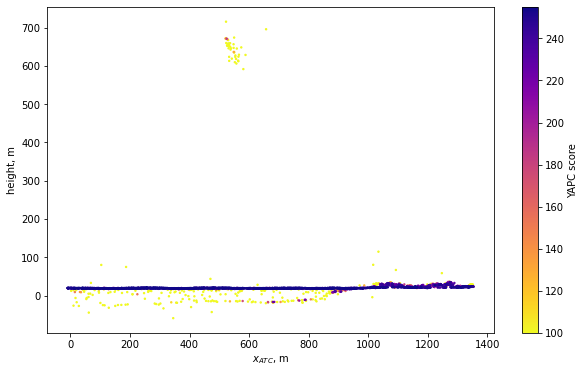
YAPC classifications
Let’s try the experimental photon classifier. See the function plot_yapc in ./coastal/plot.py. Again put a semicolon at the end to prevent the plot from showing up twice.
Once again we have this odd outlier set of photons.
plot_yapc(D3);
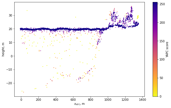
plot_yapc(D3[D3["atl08_class"] != 4], vmin=0);
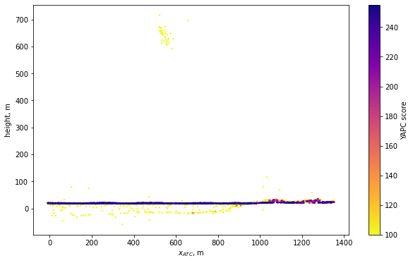
YAPC
Here I play around with changing the classification algorithm.
knn=0 is a special case where the window for the number photons is adaptive based on the total number of photons in a band.
cnf = -2 returns everything so that there is no removal of photons.
win_h = 2 and win_x = 6 will make the window smaller (looking at icebergs)
%%time
parms2 = parms
parms2['yapc'] = dict(knn=0, win_h=1, win_x=12, min_ph=0, score=0)
gdf2 = icesat2.atl03sp(
parms2,
asset=asset,
version=release,
resources=granules_list)
beam_type = 'strong'
project_srs = "EPSG:26912+EPSG:5703"
D3 = reduce_dataframe(gdf2, cycle=5, rgt=38, track=3, beam='strong', crs=project_srs)
CPU times: user 966 ms, sys: 48.4 ms, total: 1.01 s
Wall time: 1.78 s
plot_yapc(D3);
Summary
This notebook shows how to
Plot a region on a map
Get the ICESat-2 data available with SlideRule
Show the ATL08 and YAPC photon classifications
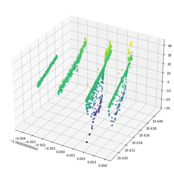
Extras 3D plots
This is just a simple 3D plot of the data in a region.
from mpl_toolkits import mplot3d
import numpy as np
import matplotlib.pyplot as plt
fig = plt.figure(figsize=(10, 10))
ax = plt.axes(projection='3d')
test = gdf[gdf["atl08_class"] != 4]
# Data for three-dimensional scattered points
zdata = test['height']
xdata = test.geometry.x
ydata = test.geometry.y
ax.scatter3D(xdata, ydata, zdata, c=zdata);
This is an interactive 3D plot.
import plotly.graph_objects as go
fig = go.Figure(data=[go.Scatter3d(
x=xdata,
y=ydata,
z=zdata,
mode='markers',
marker=dict(
size=1,
color=zdata, # set color to an array/list of desired values
colorscale='Viridis', # choose a colorscale
opacity=0.8
)
)])
fig.show()
# animate the 3d image. Hit the play button
x_eye = -1.25
y_eye = 2
z_eye = 0.5
fig.update_layout(
title='Hit the Play Button to Rotate',
width=600,
height=600,
scene_camera_eye=dict(x=x_eye, y=y_eye, z=z_eye),
updatemenus=[dict(type='buttons',
showactive=False,
y=1,
x=0.8,
xanchor='left',
yanchor='bottom',
pad=dict(t=45, r=10),
buttons=[dict(label='Play',
method='animate',
args=[None, dict(frame=dict(duration=5, redraw=True),
transition=dict(duration=0),
fromcurrent=True,
mode='immediate'
)])
])])
def rotate_z(x, y, z, theta):
w = x+1j*y
return np.real(np.exp(1j*theta)*w), np.imag(np.exp(1j*theta)*w), z
frames=[]
for t in np.arange(0, 6.26, 0.1):
xe, ye, ze = rotate_z(x_eye, y_eye, z_eye, -t)
frames.append(go.Frame(layout=dict(scene_camera_eye=dict(x=xe, y=ye, z=ze))))
fig.frames=frames
fig.show()