Slide Rule example

From the SlideRule documentation, “SlideRule is a web service for on-demand science data processing, which provides researchers and other Earth science data systems low-latency access to customized data products using processing parameters supplied at the time of the request. SlideRule runs in AWS us-west-2 and has access to the official ICESat-2 datasets hosted by the NSIDC.” See the documentation for installation instructions.

Step 1: Install packages

import matplotlib.pyplot as plt
from sliderule import icesat2
from ipyleaflet import Map, GeoData, LayersControl,Rectangle, basemaps, basemap_to_tiles, TileLayer, SplitMapControl, Polygon

---------------------------------------------------------------------------
ModuleNotFoundError                       Traceback (most recent call last)
Input In [1], in <cell line: 1>()
----> 1 import matplotlib.pyplot as plt
      2 from sliderule import icesat2
      3 from ipyleaflet import Map, GeoData, LayersControl,Rectangle, basemaps, basemap_to_tiles, TileLayer, SplitMapControl, Polygon

ModuleNotFoundError: No module named 'matplotlib'

Import the functions from our coastal library. The library is at ../ so we need to append that to the Python path.

import sys
sys.path.append('../')
from coastal.beam import reduce_dataframe
from coastal.plot import plot_atl08, plot_yapc

Step 2: Initialize the icesat2 package

icesat2.init("icesat2sliderule.org", verbose=True)

Step 3: Create a list of coordinates

Here we will import a geojson file that represents the White Mountain, Alaska region of interest. Our geojson file looks like so

{"type":"FeatureCollection","features":[{"type":"Feature","properties":{},"geometry":{"type":"Polygon","coordinates":[[[-163.16619873046875,64.4064312702572],[-162.75421142578125,64.34823209154665],[-162.77893066406247,64.54607936653424],[-163.3062744140625,64.79518717004242],[-163.69903564453122,64.69910544204765],[-163.16619873046875,64.4064312702572]]]}}]}

We have this saved to a file whitemountain.geojson.

# import the map.geojson file representing the ROI
spatialExtent = icesat2.toregion('data/whitemountain.geojson')["poly"]

# check the format of the coordinates
spatialExtent

[{'lon': -162.75421142578125, 'lat': 64.34823209154665},
 {'lon': -162.77893066406247, 'lat': 64.54607936653424},
 {'lon': -163.3062744140625, 'lat': 64.79518717004242},
 {'lon': -163.69903564453122, 'lat': 64.69910544204765},
 {'lon': -163.16619873046875, 'lat': 64.4064312702572},
 {'lon': -162.75421142578125, 'lat': 64.34823209154665}]

# create bounding box
bb = [spatialExtent[0]['lon'], spatialExtent[0]['lat'], 
      spatialExtent[2]['lon'], spatialExtent[2]['lat']]

# create polygon for plotting
polygon = Polygon(
    locations=spatialExtent,
    color="green"
)

Step 4: Visualize region of interest

center = [spatialExtent[0]['lat'], spatialExtent[0]['lon']]
zoom = 8
m = Map(basemap=basemaps.Esri.WorldImagery, center=center, zoom=zoom)
m.add_layer(polygon);
m

Step 5: Create a dictionary of processing parameters

These will specify how the elevations (from ATL03 photon data) for the region should be calculated.

%%time

# build sliderule parameters for ATL03 subsetting request
# SRT_LAND = 0
# SRT_OCEAN = 1
# SRT_SEA_ICE = 2
# SRT_LAND_ICE = 3
# SRT_INLAND_WATER = 4
parms = {
    # processing parameters
    "srt": icesat2.SRT_LAND,
    "len": 20,
    # classification and checks
    # still return photon segments that fail checks
    "pass_invalid": True, 
    # all photons
    "cnf": -2, 
    # all land classification flags
    "atl08_class": ["atl08_noise", "atl08_ground", "atl08_canopy", "atl08_top_of_canopy", "atl08_unclassified"],
    # all photons
    "yapc": dict(knn=0, win_h=6, win_x=11, min_ph=4, score=0), 
}

CPU times: user 5 µs, sys: 1e+03 ns, total: 6 µs
Wall time: 8.58 µs

Set the data asset, release and time boundaries for query

# Set ICESat-2 data asset
asset = "nsidc-s3"

# ICESat-2 data release
release = '005'

# time bounds for CMR query
time_start = '2019-07-10'
time_end = '2019-07-20'

Step 6: Find the granules

This code will find the granules, create an empty geodataframe and write the query into the geodataframe.

# find granule for each region of interest
granules_list = icesat2.cmr(polygon=spatialExtent, time_start=time_start, time_end=time_end, version=release)

# create an empty geodataframe
parms["poly"] = spatialExtent

# write output into geodataframe
gdf = icesat2.atl03sp(parms, asset=asset, version=release, resources=granules_list)

INFO:sliderule.icesat2:Allocating 21 workers across 7 processing nodes
INFO:sliderule.icesat2:0 points returned for ATL03_20190710014600_01830405_005_01.h5 (1 out of 3 resources)
INFO:sliderule.icesat2:1361414 points returned for ATL03_20190714013741_02440405_005_01.h5 (2 out of 3 resources)
INFO:sliderule.icesat2:874960 points returned for ATL03_20190718012923_03050405_005_01.h5 (3 out of 3 resources)

# look at the resulting geodataframe
gdf.head()

	segment_id	segment_dist	track	cycle	rgt	sc_orient	delta_time	atl03_cnf	height	distance	atl08_class	yapc_score	quality_ph	pair	geometry
time
2019-07-14 01:41:43.864015240	642346	1.286611e+07	3	4	244	0	4.830370e+07	0	167.423950	-8.519688	4	0	0	0	POINT (-162.95389 64.62952)
2019-07-14 01:41:43.864015240	642346	1.286611e+07	3	4	244	0	4.830370e+07	0	-0.217391	-3.846664	4	0	0	0	POINT (-162.95390 64.62948)
2019-07-14 01:41:43.864015240	642346	1.286611e+07	3	4	244	0	4.830370e+07	0	-187.967499	1.387081	4	0	0	0	POINT (-162.95392 64.62943)
2019-07-14 01:41:43.864015240	642346	1.286611e+07	3	4	244	0	4.830370e+07	0	-216.398285	2.179764	4	0	0	0	POINT (-162.95393 64.62943)
2019-07-14 01:41:43.864015240	642346	1.286611e+07	3	4	244	0	4.830370e+07	0	-271.506531	3.715942	4	24	0	0	POINT (-162.95393 64.62941)

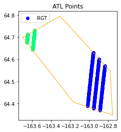
Step 7: Plot the Reference Ground Tracks

The RGT is an imaginary line through the six-beam pattern that is handy for getting a sense of where the orbits fall on Earth, and which the mission uses to point the observatory. For more information see the ICESat-2 description here.

# get unique RGTs
rgtValues = gdf['rgt'].unique()
rgtValues.sort()
print(rgtValues)

[244 305]

Plot the output by RGT track within the region of interest

f, ax = plt.subplots()
ax.set_title("ATL Points")
ax.set_aspect('equal')
# FIX THIS TO SHOW EACH RGT value by color
gdf2 = gdf.sample(n=1000, replace=False, random_state=1)
gdf2.plot(ax=ax, column='rgt', label='RGT', c=gdf2['rgt'], cmap='winter')
ax.legend(loc="upper left")
# Prepare coordinate lists for plotting the region of interest polygon
region_lon = [e["lon"] for e in spatialExtent]
region_lat = [e["lat"] for e in spatialExtent]
ax.plot(region_lon, region_lat, linewidth=1, color='orange');

center = [spatialExtent[0]['lat'], spatialExtent[0]['lon']]
zoom = 8
m2 = Map(basemap=basemaps.Esri.WorldImagery, center=center, zoom=zoom)
m2.add_layer(polygon);
geo_data = GeoData(geo_dataframe = gdf.sample(n=1000, replace=False, random_state=1),
    style={'color': 'red', 'radius':1},
    point_style={'radius': 1, 'color': 'red', 'fillOpacity': 0.8},
    name = 'rgt')
m2.add_layer(geo_data)

m2

Step 9: Reduce GeoDataFrame to plot a single beam

We also want to convert coordinate reference system to compound projection. First let’s see what is in our data.

df = gdf[['cycle', 'track', 'pair', 'sc_orient']]
for cyl in gdf['cycle'].unique():
  tmp = gdf[gdf['cycle']==cyl];
  for track in tmp['track'].unique():
    tmp2 = tmp[tmp['track']==track];    
    for rgt in tmp2['rgt'].unique():
       print('cycle=', cyl, ', track=', track, ', rgt=', rgt)

cycle= 4 , track= 3 , rgt= 244
cycle= 4 , track= 2 , rgt= 244
cycle= 4 , track= 2 , rgt= 305
cycle= 4 , track= 1 , rgt= 244
cycle= 4 , track= 1 , rgt= 305

We need to pick one of these.

beam_type = 'strong'
project_srs = "EPSG:26912+EPSG:5703"
D3 = reduce_dataframe(gdf, cycle=4, rgt=305, track=2, beam='strong', crs=project_srs)

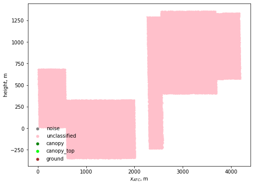
D3["atl08_class"].value_counts()

4    150263
0        41
Name: atl08_class, dtype: int64

Class 4 is unclassified. It looks like our data are unclassified (4) or noise (0).

plot_atl08(D3);

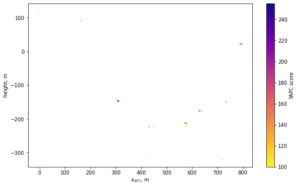
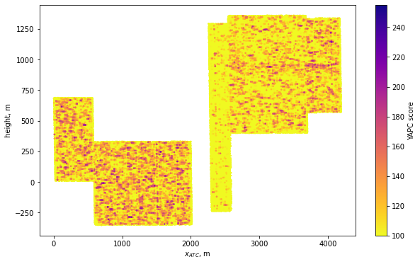
Plot YAPC

plot_yapc(D3);

plot_yapc(D3[D3["atl08_class"] != 4]);